Interpretation tools

Interpretation tools work on both point cloud and on surface mesh data. They are available via the Interpretations tab in the Ribbon Bar, which is divided into five panels:

• Navigation — get back to plain camera movement, or pick a standard view.
• Active Descriptor — the facies and horizon pick applied to everything you digitise next.
• Structure — orientations, faults, scan lines, plunges and polylines.
• Sedimentology — geopolygons, palaeocurrents, sedimentary logs and boreholes.
• Edit — fix up what you have already digitised.

Annotations — scale bars, measurements, labels and the rest — sit on their own ribbon tab next door.

The full reference is next door

This page walks you through the main tools. The Basic Interpretation guide covers the same ground in more depth — every digitising mode, the Active Descriptor, Sticky Interp and Pause Digitising, scan lines, and what to do with an object once you have made one.

Two habits worth forming early

Sticky Interp (on the Structure panel) keeps a tool armed after each object, so you can digitise many features without returning to the ribbon. Pause Digitising (on the Edit panel) suspends a part-finished line so you can navigate, then resumes it — it does not end the line.

1. Structure Panel

This Structure Panel includes several methods of collecting structural information from a 3D outcrop. Most of the tools have a sub-menu of digitising modes, described below.

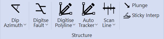
1. Planes (Dip Azimuth)
2. Faults
3. Polylines
4. Auto Tracker
5. Scan Lines
6. Plunges
7. Sticky Interp

Dip Azimuth (orientations or planes)

This tool records a planar orientation. The Dip Azimuth button carries five methods of collecting one, and the choice matters:

No.	Type	Definition	Usage
1.	3 Points	Default when Dip Azimuth is selected. A best-fit plane is created from 3 selected points.	Click 3 points on the 3D model to calculate an orientation.
2.	N points	N-Points method allows n number of points to be digitised.	Click n number of points on the 3D model. Double click to end the digitisation and calculate the orientation. Equally, click + drag to automatically extract n points along the digitised trace.
3.	1 Point	1 Point method allows for a measurement to be manually entered into the model, such as a measurement taken in the field.	Click where the orientation data was collected and enter the associated Dip and Azimuth.
4.	Area	Fits one plane through every point inside a lassoed region, which is the most robust fit available. Point clouds only.	Choose Area, then drag a freehand lasso around the exposed surface. The plane is fitted when you release.
5.	Attributes	Reads the orientation straight from a mesh that has already been analysed for dip and azimuth.	Click a point on the analysed mesh.

Whichever method you use, the result is an orientation object in the Interpretations tree, plotted on the stereonet and usable by every downstream tool.

Orientations are classified after the fact, not by picking a mode first. Select one or more in the Interpretations tree, then right + click → Classification and choose Bed, Fracture, Cleavage, Foreset or Regional. The classification drives how they are drawn and how the stereonet groups them.

 

Polylines and Faults

Polylines and Faults share the same digitising modes and are executed in the same way.

This section describes the polyline digitising and editing facilities. Both Digitise Polyline and Digitise Fault have sub-menus of different methods to digitise the desired feature. After successful addition of a Polyline or Fault, metadata may be added such as the Stratigraphy where the feature is located. The default option creates a new object of that type.

Type	Definition	Usage
Digitise Polyline	Creates a 3D polyline from digitised points	Points are digitised by individual clicks on the model, or click + drag to continually digitise*. Double click ends digitisation. Single click digitising is default behaviour.
Digitise Fault	Creates a 3D polyline from the digitised points of a fault feature.	Similar to Polylines, points are digitised by individual clicks on the model, or click + drag to continually digitise*. Double click ends digitisation. Single click digitising is default behaviour.

Faults

The Digitise Fault sub-menu carries the fault-specific operations:

Type	Definition
New Fault	Start a new fault.
Split	Split a fault into two at a chosen vertex.
Join	Join two faults into one.
Add stick	Add another fault stick to the same fault object, which is how a fault surface is built up across a series of exposures.
Extend Fault	Continue digitising an existing fault from its end.

Polylines

There are several options to modify and edit a digitised Polyline and even combine multiple Polylines. Click to expand the Digitise Polyline menu to reveal the sub-menu. In this menu, you can perform several functions:

Type	Definition	Usage
Digitise Points	The default. Build the Polyline from individual clicks.	Click each point in turn; double click to end.
Draw	Freely draw the Polyline	Click + drag to freely draw the position and length of the Polyline on the outcrop model.
Draw Contour	Digitise a line of constant elevation across the model.	Pick a point at the elevation you want and the contour is traced from it.
Geodesic Distance	Digitise a line that follows the shortest path across the surface between your clicks, with a live along-surface length readout.	Click sparse points along the feature. Because the line stays on the rock instead of cutting through it, this is the right tool for measuring along an undulating surface.
Split Line	Split Polyline into multiple Polylines.	This function is performed at vertices. Click the Polyline to activate and make vertices visible. Click the desired vertex where you'd like to split the Polyline. The Polyline will be split in two and the new Polylines will appear in the interpretation tab.
Join Lines	Join multiple Polylines together. Creates one Polyline.	Hold ctrl and click the Polylines to join together. When all Polylines are selected, choose the Join Lines menu option to combine all selected Polylines.
Add Node	Add a node to a selected Polyline	Select a Polyline to activate it. Simply click anywhere along the Polyline length to add a node at that location. Add as many nodes as you'd like. Select the Add Node menu option to finish and save newly added nodes.
Close Polyline	Joins the last node back to the first, making a closed loop.	Select the Polyline, then choose Close Polyline.
Snap To Mesh	Drops every node of the Polyline onto the mesh surface.	Useful after translating a line, or when a line digitised against one object needs to follow another.
Create Geobody	Creates a new Geopolygon from the selected Polylines.	Select multiple polylines so they are active. Choose Create Geobody menu option to create the new Geopolygon. This is stored in the Geopolygon Interpretations group.

 

Polyline right-click menu

There are other Polyline editing options, reached by right + click on the Polyline in the Interpretations Tree. They are grouped into sub-menus; the most commonly used are:

No.	Sub-menu	Type	Definition	Usage
1.	Quality & Refinement	Refine by Spacing	Reduce the number of nodes for the given Polyline by user-defined distance.	If chosen, a dialogue box appears. Simply enter the desired distance, in metres, between nodes along the polyline length.
2.	Quality & Refinement	Smooth	Smooth the Polyline, removing digitising jitter.	Useful after freehand Draw digitising.
3.	Quality & Refinement	Adaptive Refine	Add nodes where the line curves and leave straight runs alone.
4.	Attributes	Remove Dip	Remove the best-fit Dip value from the Polyline.	If chosen, a dialogue box is displayed that allows you to enter desired Dip value to remove from the Polyline.
5.	Attributes	Calculate Best Fit Plane	Fit a plane through the Polyline and record its dip and azimuth.
6.	Transform	Translate	Translate polyline in any x, y, z direction.	If chosen, a dialogue box is displayed with separate x, y, z text fields. Enter the desired amount to translate the Polyline.
7.	Transform	Attach to Visible Meshes	Drop the Polyline onto the visible mesh surface.
8.	Convert To	Orientation	Turn the Polyline into an orientation measurement.

The complete menu is listed in the Polylines tree reference.

Other Polyline and Fault editing tools

You can Edit Polylines and Faults during and after creation.

There are several options to edit a Polyline or Fault.

• Move Vertices
• Pause Digitising
• Undo
• 3D Translate
• Snap Vertices
• Erase Vertices
• Reposition Object

No.	Type	Definition	Usage
1.	Move Vertices	Freely move a chosen vertex to any position	Click the desired Polyline or Fault. The nodes will appear. Choose Move Vertices from the Edit bar and click + drag the vertex to the next desired position. Click Move Vertices again to save new vertex position. N.B. you can select a vertex before selecting Move Vertices this vertex will be the updated one when you click the new position. To de-select a vertex simply click on it again while not in an editing mode.
2.	Pause Digitising	Pause active Polyline or Fault digitising session.	Whilst digisiting a Polyline or Fault, click Pause Digitising to momentarily pause digitising. This allows you to navigate around the 3D model around. Click Pause Digitising again to resume the digitising session.
3.	Undo	Undoes last action	When drawing a Polyline or Fault, click this to Undo the digitisation.
4.	3D Translate	Move a Polyline or Fault vertex along x,y,z axes	Click on Polyline or Fault to make active. Choose 3D Translate and click on the node that you wish to move. Choose the axis arrows You can either move the node along the x, y, or z axis. Click + drag the plane along those axes allows free movement along that plane's orientation.
5.	Snap Vertices	Snaps digitised vertex to existing vertex nearby
6.	Erase Vertices	Erases selected vertices of Polyline or Fault	Click to activate a Polyline or Fault and display its vertices. Simply click the vertex you want to erase to erase it.
7.	Reposition Object	Move a whole interpretation object to a new place on the model	Select the object, choose Reposition Object, then click where it should sit. Handy when an orientation or annotation was picked slightly off the feature it describes.

Auto Tracker

Rather than clicking along a feature, Auto Tracker follows it across the mesh for you: give it a start and an end and it finds the path between, guided by the mesh's own attributes. Settings on its sub-menu puts the tracker's parameters in the Properties Panel.

OpenGL view only

The Auto Tracker is handled by the OpenGL view. In a Vulkan view the button is inert — use Geodesic Distance for surface-following traces, or switch renderer in Project Properties.

Scan Lines

A Scan Line samples fracture intensity along a line, the way a tape across the outcrop does in the field. There are two ways to build one:

Type	Definition
From intersections	Digitise the line; VRGS intersects it with the orientations already displayed and records where each one crosses.
From Points	Digitise the line, then mark each fracture position along it by hand.

Both need at least two points and finish on a double click. The result feeds fracture-intensity analysis and DFN work.

Lineation and Plunges

The Plunge, or lineation, tool is very simple. Select a start and end point for a lineation on the model and VRGS calculates the Dip and Dip direction of the line. Additionally, VRGS automatically calculates the Plunge of a Fault that is digitised on a 3D model.

 

2. Sedimentology Panel

VRGS has several tools key to analysing sedimentary features in 3D outcrop models. The tools included in the Sedimentology section are:

1. Geo Polygon (e.g. geobodies)
2. Measured Section (sedimentary logs) — see the Sedimentary Logging guide
3. Palaeocurrent
4. Borehole

Type	Definition	Usage
Geopolygon	Create a Geopolygon outline around interpreted geobodies and extrude it as a solid object away from the outcrop model. Attributes such as Dip and Dip Azimuth and Palaeocurrents may be added to the object to allow further statistics to be measured from it.	Select the Geo Polygon tool and click or click + drag the mouse to digitise points along the outcrop. Double click will end digitisation. At least three points are needed, and the outline is closed for you.

Its sub-menu carries the other ways in: Digitise Points (one vertex per click), Draw (freehand), Key Pillar (a pillar controlling the extrusion), and Create from polylines (build the outline from lines you have already digitised). The Geopolygon guide covers the extrusion and the statistics in full.

A facies name may be added to the Geopolygon. To do this select the active facies from the Active Descriptor drop-down at the left of the Interpretations ribbon tab — everything you digitise next inherits it. The Apply to selected item on the same drop-down stamps the active facies onto objects you have already made, and a second drop-down does the same for the active horizon pick. Additional facies can be added through the Facies group in the Collections Tree. Once a Geopolygon has been digitised then extended features can be made available by right + click on the Geopolygon in the Interpretations Tree and selecting Make Active. This will provide editing focus to the selected Geopolygon. A new Ribbon Bar will appear in the top menu.

Editing Geopolygons

There are 3 main editing functions for Geopolygons

• Move
• Select Nodes
• Move Nodes

Type	Definition	Usage
Move	Return to normal model interaction, or Move mode	This quits any active editing to the Geopolygon
Select Nodes	Show all the digitised vertices of the geobody as spheres.	Click on one or more spheres to select them. You can then delete them by pressing the Delete key.
Move Nodes	Move selected nodes	Select a node then click the point on the model you wish to move it to.
Interpolate Nodes	Add node by interpolation between selected nodes	Select adjacent nodes on the Geopolygon and a new node will be interpolated between them.
Add Palaeocurrent	Add multiple palaeocurrent measurements to a Geopolygon.	Select Add Palaeocurrent and a dialogue box will appear. You can add a recorded palaeocurrent value in the Azimuth text field. Indicate if it's a bi-directional measurement, such as a trend rather than a known direction. You can and even provide a type (e.g. trough cross-bedding, current ripple cross lamination, etc). Palaeocurrent types are added in the Collections Tree in the Sed Structures menu. To delete a measurement, select the value in the list then press Delete. Right + click on the Geopolygon and select Make Active again to switch off active editing.

Notes about sedimentary Geopolygons

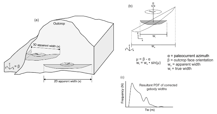
Geopolygons can encapsulate a large rock volume, and it is often the case in sedimentary systems that there is variability in the palaeocurrent directions. We can record this variability by adding those palaeocurrents in the Geopolygon. Outcrops are inherently biased by sedimentary system architecture - the geometry observed on the outcrop exposure is a function of the exposure level and related weathering. However, adding palaeocurrent values to interpreted Geopolygons we can correct for this bias¹,². These can then be used to calculate corrected sedimentary body widths. See the image below for a graphical representation of how Geopolygon widths are corrected using palaeocurrent data from outcrop³.

Footnotes

1. Fabuel-Perez, I., Hodgetts, D. and Redfern, J., 2010. Integration of digital outcrop models (DOMs) and high resolution sedimentology–workflow and implications for geological modelling: Oukaimeden Sandstone Formation, High Atlas (Morocco). Petroleum Geoscience, 16(2), p.133-154. https://www.lyellcollection.org/doi/abs/10.1144/1354-079309-820 ↩

2. Rarity, F., Van Lanen, X.M.T., Hodgetts, D., Gawthorpe, R.L., Wilson, P., Fabuel-Perez, I. and Redfern, J., 2014. LiDAR-based digital outcrops for sedimentological analysis: workflows and techniques. Geological Society, London, Special Publications, 387(1), p.153-183. https://www.lyellcollection.org/doi/full/10.1144/SP387.5 ↩

3. Burnham, B.S. and Hodgetts, D., 2019. Quantifying spatial and architectural relationships from fluvial outcrops. Geosphere, 15(1), p.236-253. https://pubs.geoscienceworld.org/gsa/geosphere/article/15/1/236/567741/Quantifying-spatial-and-architectural ↩